Fast gas injection system for plasma physics experiments [a]

S. C. Bates* and K. H. Burrell**

* Thoughtventions Unlimited LLC, 40 Nutmeg Lane, Glastonbury, CT

** GA Technologies Inc., San Diego, CA

A system has been developed for fast, feedback controlled injection of hydrogen and various other gases into a vacuum system. Gas flow is through short (about 30-mm length), submillimeter diameter tubing at pressures in the fluid flow regime. The flow is controlled by a piezoelectric valve and measured by a miniature pressure sensor mounted in the body of the valve. Flow rates from a single valve of up to 500 Torr liter/s for hydrogen have been obtained. Response time of the flow is a rise time of 0.5 ms (with a 3-ms ringing decay time) and a fall time of 0.3 ms. The flow rate is basically a linear function of the measured pressure. A model has been developed to explain the observed functional dependence of flow rate on pressure, gas type, and tube radius.

INTRODUCTION

Pulsed hydrogen gas injection has been used quite successfully over the last ten years to control plasma density in fusion research devices such as tokamaks. Systems for such injection have grown in sophistication from ones producing constant flow rates to fast, feedback controlled units that can match almost any arbitrary, preprogrammed wave shape [1,2]. Gas injection has also been used for the injection of gaseous impurities to study plasma transport properties. As larger devices are constructed, the hydrogen flow rate requirements increase. In addition, impurity injection requires short time responses. Finally, the advent of reversed field pinch devices with their short pulses (< 20 ms) and high throughput requirements have added to the need to develop a fast response (< 1 ms), high throughput (< 500 Torr liter/s) gas injector. The present work is a report on the design and testing of such an injector.

The current injector evolved out of previous work [1] on feedback controlled gas injection systems. Like that system,[1] the current one uses high-pressure (0.1 to 2.0 bar) flow in a submillimeter diameter tube to achieve rapid time response. Flow rate is measured by means of a small pressure sensor mounted in the body of the piezoelectric gas valve, which controls the flow. The pressure sensor signal is used for feedback control of the valve.

The current system has an overall gas flow length of only 30 mm, which is considerably shorter than the previous system [1]. Consequently, it has much faster time response: rise time is 0.5 ms and fall time is 0.3 ms. A hydrogen throughput of up to 500 Torr liter/s has been achieved. (Exploiting the full capability of such a valve on a given vacuum system requires ports with quite good conductance; otherwise, pulse broadening due to port conductance limitations will occur.)

We present the design in Sec. 1, followed by a discussion in Sec. II of the important physical effects controlling the flow. Our experimental investigation of the effect of pressure, gas type, tube length, and tube radius on the total throughput is given in Sec. III. The results fit the model of Sec. II reasonably well.

I. DESIGN

If we consider gas flow in the viscous, Poiseuille flow regime, it is easy to show' that the time response of the flow scales as l, [3],[2] where l is the overall tube length. For a given pressure, throughput Q also increases as l is made shorter. Accordingly, the current design stresses achieving minimum length consistent with the constraint imposed by the presence of the pressure sensor used for flow measurement and control. The result is shown in Fig. 1.

The viscous flow tube has been built into a standard piezoelectric valve (Veeco PV-10) along with inserts that fill extraneous volume. The tube radius a is 0.36 mm; the distance from the pressure sensor tip to the output end is about 12.5 mm. The pressure sensor (ENTRAN Devices EXP-1032) has been inserted into the valve body with its tip as close as possible to the flow passage to minimize trapped volume.

When we thoroughly tested the flow versus pressure behavior of the injector shown in Fig. 1, it was clear that although it met all desired specifications on flow rate and rise time, it did not behave as the Poiseuille flow equations would have predicted. As we will see presently, the tube had been shortened to the point that Poiseuille flow does not have space enough to develop. In order to understand the observed behavior, we embarked on a series of parametric tests and a much more thorough theoretical investigation.

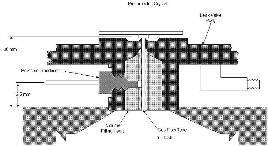
FIG. 1. Drawing of the fast response, viscous flow gas injector. This is a highly modified Veeco PV-10 piezoelectric valve. The pressure sensor is ENTRAN EPX-1032, which has a tip the size of a 10-32 screw. The injector is welded into a 2 3/4 in. conflat flange.

II. FLOW EQUATIONS

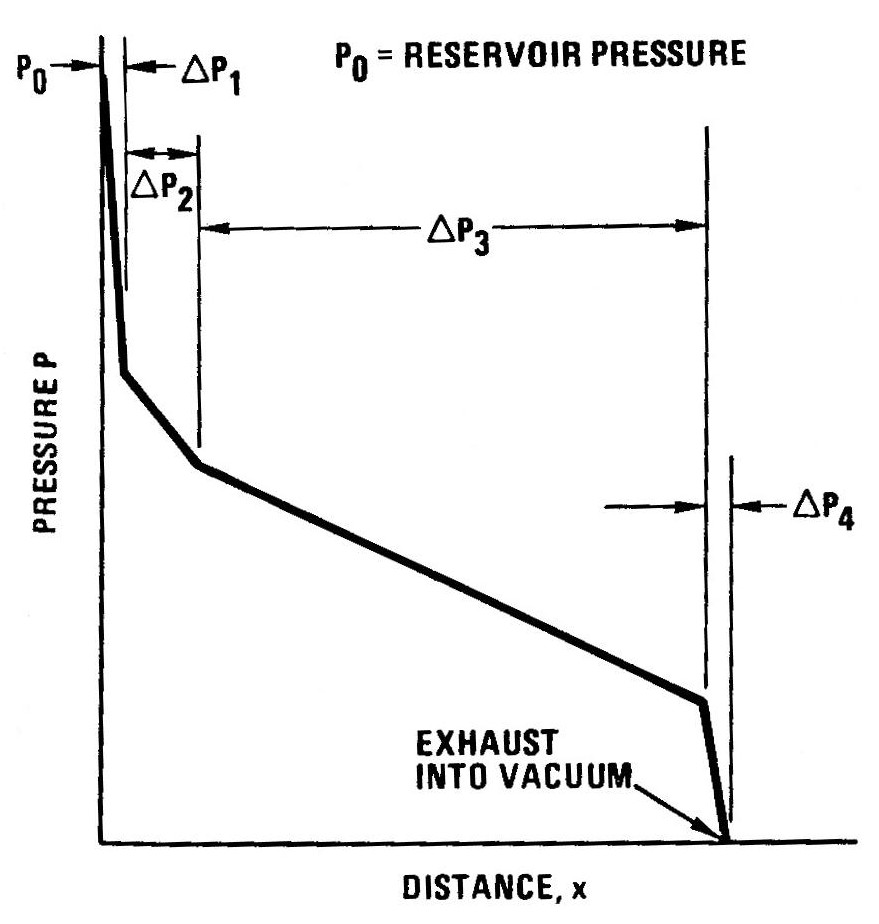
Fig. 2. Pressure variation down a viscous flow tube injector. δP₁ is the pressure drop across the piezoelectric valve, δP₂, is the pressure drop in the region of developing flow, δP₃, is the fully developed (Poiseuille flow) pressure region, and δP₄, is the pressure drop across the sonic orifice at the end of the tube.

For any fluid handling system the flow rate adjusts itself to give a pressure drop in the system equal to the difference between the entrance and exit pressures. The case of a viscous flow tube injector can be idealized as shown in Fig. 2. It consists of a reservoir, a constriction (valve), a resistive viscous flow section, and an exhaust into vacuum. Measuring the pressure at some position down the tube, as is done for the purposes of valve feedback control, completely specifies the flow rate of the injector. For this reason the equations describing the viscous flow tube injector relate the flow rate to the pressure drop from the transducer position down stream to the vacuum chamber.

At the upstream end of the tube flow is spatially uniform with a velocity u related to the mass flow rate Q_m by the continuity equation

u = Q_m/ρA (1)

where ρ is the gas density and A is the tube cross-sectional area. As the gas moves downstream, viscous boundary layers grow on the wall dissipating energy and causing a pressure drop. Since the flow rate must remain constant for steady low, as viscosity slows the gas near the wall the potential low core of uniform velocity must accelerate so that the mean velocity ū now satisfies Eq. (1). Although a complete description of this developing flow is only susceptible to numerical analysis, a simple estimate of the effects of the boundary layer can be made.

The boundary layer thickness δ * on a flat plate grown as [3]

δ * = 1.72 (νx/U)^1/2 = 1.72x/(Re_x), (2)

where U is the free stream velocity, νη/ρ is the kinematic viscosity, η is the coefficient of viscosity, x is the distance downstream, and Re = ρU_x/ η is the Reynolds number based on the length x. δ* is the displacement, or momentum thickness of the layer, appropriate to the constriction and acceleration of the uniform core flow. Similarly, the shear stress, σ, along the plate is

σ = 0.33 (ηρU³/x)^1/2 (3)

For the pipe flow considered here, Eq. (2) indicates that as the core, or free stream, flow accelerates due to the constriction, the boundary layer growth rate will decrease. The boundary layer thickness will grow as √x until the core is restricted (i.e., δ*/α is significant), then δ* grows more slowly. In the tube, we have

σ = 0.57 (ηU/ δ*) ≈- (α./2)(dp/dx) (4)

and

dp/dx = - (2/α)(0.57)(ηU/δ*) (5)

The pressure drop per unit length should be approximately constant, as the core flow accelerates, since δ* grows slowly.

Equations (2)-(5) give an estimate of the thickness of the boundary layer in the tube and the pressure drop resulting from it. The boundary layer grows down the tube until either the tube ends or it is completely filled by the viscous layer. In this latter case, the flow eventually relaxes to a constant velocity profile with viscosity important throughout the tube. This flow is known as Poiseuille flow.

In Poiseuille flow, the pressure drop along the pipe ∆p is related to the pipe parameter [4] as

∆p = 8ηūl/α² (6)

The pressure drop along the pipe is

dp/dx = - 8ηū/α² = - 8ηQ_m/πρa⁴ (7)

If we assume that the flow is at constant temperature, then p is linearly related to ρ through p = ρR T, where R = R/, R is the universal gas constant and m is the molecular weight. Using this and integrating Eq. (7), we find

p² = (l6ηQ_ml /πα⁴)RT (8)

where we have assumed that the exit pressure is zero. Note that the flow acceleration due to the pressure drop along the pipe is included as a 1/ρ term in Eq. (7).

If the length of tube where the boundary layer grows is short compared to the overall length, then the pressure drop will be described by the Poiseuille flow Eqs. (6)-(8). The length of tube required for transition to Poiseuille flow has been calculated by Langhaar,[5] for a laminar, incompressible, constant density flow. The flow was found to develop as a function of the parameter σ^t= x/D Re_D, where D = 2a is the tube diameter and Re_D = ρUD/η is the Reynolds number based on that diameter. The approximate length to transition

1_t= 0.227aRe_D (9)

The flow is in the early stages of transition if σ_t « 1. This analysis includes the acceleration of the flow due to constriction by the boundary layer, but does not include the acceleration due to the dropping density as the pressure decreases down the tube. Thus, this estimate is a lower limit in the present case.

When considering the pressure drop of fully developed pipe flow, the Reynolds number must be small enough to ensure laminar flow. Otherwise the pressure drop is significantly higher due to turbulence. In fully developed pipe flow the transition to turbulence occurs at a critical Reynolds number of about 2,100.

Re_т = ρuD/η ≈ 2100. (10)

The transition to turbulence is directly proportional to the flow rate Q. However, when the tube is too short to permit full flow development, the critical Re_т can be much higher.

Finally we consider what happens at the end of the tube, where the gas expands and accelerates into vacuum. Independent of the state of the fluid in the tube, the end of the tube acts as a sonic orifice, since the pressure drop to vacuum is always greater than the factor of 2 necessary for sonic flow. For any sonic orifice, we have the mass flow rate given by [6]

Q_m = p₀A_t ( γ/RT₀ )^1/2 (2/( γ + 1)) ^{(γ+1)/2(γ-1)} (11)

where p₀ is the stagnation pressure behind the orifice, A, is the effective throat area, γ is the ratio of specific heats, and T_o is the stagnation temperature. The effective throat area is the true area of sonic flow, which is less than the physical cross section due to the boundary layer on the wall. The area reduction can be quite significant for an orifice where boundary layer thickness is comparable to its radius, as is the case here. The pressure required to drive the sonic flow is a linear function of the flow rate, such that for low flow rates of Poiseuille flow this contribution to the pressure drop is negligible. However, it will be shown that this effect dominates for the high flow rate tube injectors considered here.

Note that the quantities involved in Eq. (11) are stagnation quantities [6]. When the flow velocity exceeds about 30% of the speed of sound c_s the flow is compressible, and the pressure, temperature, and density of the fluid are significantly different when measured at rest or moving. It is then proper to speak of the static pressure, p_s and stagnation pressure p_o. The pressure transducer shown in Fig. 1 is positioned so that it measures static pressure. Relating the pressure drop to flow rate, however, is properly done in terms of the stagnation pressure. Viscous dissipation causes a drop in both static and stagnation pressure.

An additional complication of compressible flow is that thermal energy can be transferred into kinetic energy; hence, the equation of state is the adiabatic one, rather than the isothermal one characteristic of incompressible, Poiseuille flow. For short tubes and high flow rates, the transit time is too short for significant heat transfer. How rapidly thermal equilibration takes place compared to the relaxation to fully developed, viscous flow can be gauged by comparing thermal diffusivity α = κ/ρc_p on to the momentum diffusion ν = η/ρ. (Here, κ is the thermal conductivity and c_p is specific heat at constant pressure.) The ratio α/ν = κ/(ηc_p) is about 1.5 for hydrogen and is near unity for most gases. Accordingly, temperature and momentum boundary layers develop at the same rate. This boundary layer that grows into fully developed flow is both a momentum and a thermal boundary layer. The core flow, however, is adiabatic and a spatially uniform velocity.

For the adiabatic core flow, the equation relating to static and stagnation pressures is [6]

p_o= p_s ( 1+ (γ-1)M²/2)^γ/(γ-1)

where M = u/c_s is the Mach number.

III. EXPERIMENTAL TESTS AND COMPARISON WITH THEORY

In order to obtain enough information to match the theory in Sec. II with the behavior of the injector in Fig. 1 we found it necessary to measure the relationship between the particle throughput Q and transducer pressure p for various gases and for a whole group of similar injectors with different tube lengths and radii. As will be seen, the basic picture that emerged is that the functional form of the Q vs. p relationship is dominated by the linear behavior characteristic of a sonic orifice; however, actual magnitude of the flow reflects the growth of boundary layers on the wall of the tube.

The test apparatus consisted of a small bell jar with these various gas injectors attached directly to the 60-liter volume. Pumping was provided by a 200-liter/s oil diffusion pump. The flow rate through the gas injector was measured by Matheson linear mass flow meter calibrated for hydrogen which read 1.0 standard liter/min full scale. The pressure transducer output was amplified and read out on an oscilloscope. Calibration of the transducer output was done comparison to a Matheson mechanical pressure gauge. Data were taken at varying repetition rates and gas pulse lengths in order to minimize the error in the average flow rate measured by the mass flow meter. The flow rate and pressure measurements should both have a relative error of 3% to 4%.

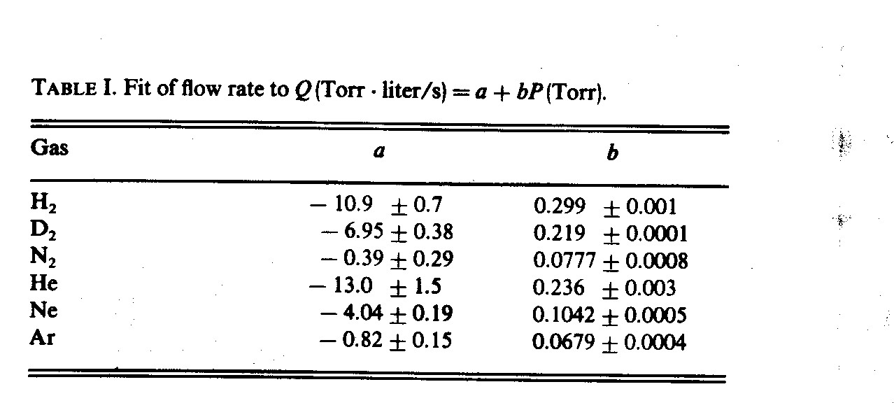
The basic hydrogen flow rate data for the injector of Fig. 1 are shown in Fig. 3. The flow rate increases approximately linearly with measured pressure over the measurement range of 17 to 500 Torr liter/s. Figure 4 contains similar data for various pure gases. These, too, fit a straight line quite well except, perhaps, at the lowest helium flow rates. The parameters of the lines of best fit in Figs. 3 and 4 given in Table 1. (On the Doublet Ill tokamak, we frequently use a copy of the current injector to inject a 90% H₂, 10% impurity gas mixture; the data in Fig. 3 should be approximate for such mixtures.)

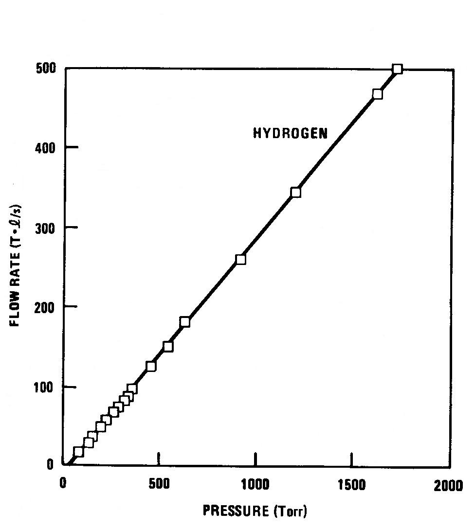
Figure 3. Hydrogen flow rate vs pressure for the gas injector in Fig.1. Maximum throughput achieved is 500 Torr liter/s with 6.5 bar behind the valve and an operating voltage of 175 V.

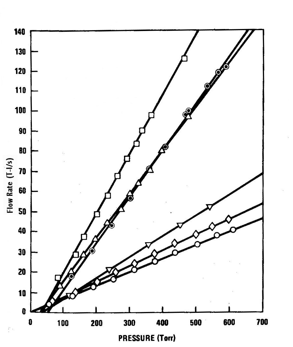
Figure 4.Flow rate vs pressure for various pure gases. See Table I for the parameters of the lines of best fit.▼Ĕ ▼- Neon; Ο--argon; ● - helium; X -- oxygen; ◊- hydrogen; ∆ - deuterium.

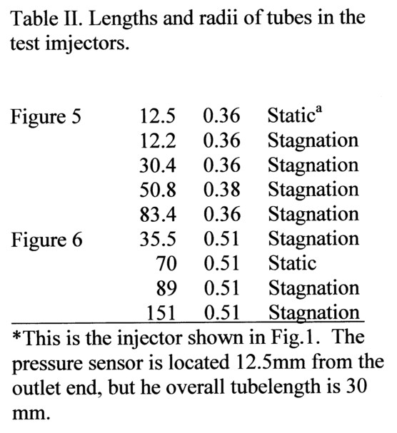
The data showing the effects of radius and length variation on hydrogen flows are presented in Figs. 5 and 6. Most of the tests were done by attaching different pieces of tubing to a tee with a pressure transducer mounted in it. The gas is fed into the tee by a piezoelectric valve; the internal volume of the tee is large enough that the transducer measures stagnation pressure. Table II gives the tube lengths and radii used.

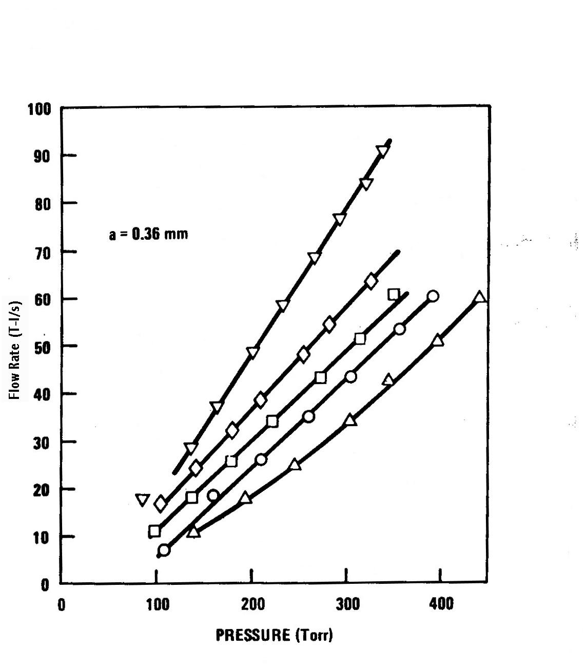
Figure 5. Flow rate vs pressure for various tube lengths but constant tube radius (a = 0.357 mm). Pressure measured is stagnation pressure except where otherwise indicated. The static pressure curve is for the injector in Fig. 1. ▼ℓ= 12.5 mm static pressure; ◊ℓ'= 12.2 mm; □ℓ= 30.4 mm; ○ℓ= 50.8 mm; ∆ℓ= 83.4 mm.

In addition to steady-state flow measurements, we have also studied the rise and fall times of the flow. These measurements are shown in Fig. 7. Figure 7 (a) indicates an e-folding decay time of 0.3 ms after a 0.1 -ms shut-offdelay. As is shown in Fig. 7(b), the valve turn on is more complex. The initial opening of the valve results in a rise with a 0.5 -ms efolding. However, the flow shows a damped oscillation, with 1-ms period and 3-ms e-folding, due to oscillation of the piezoelectric crystal about its equilibrium position. Flexure of the crystal results in a voltage that is easily detected at the voltage terminals on the valve.

Notice that for almost all the data in Figs. 4-6, the flow rate versus pressure relation is basically linear. (The exceptions are for long tubes or low flow rates.) Recalling our discussion in Sec. I, this argues that the sonic orifice at the end of the tube is dominating the flow.

If the flow had been fully developed, Poiseuille flow, we would have expected a Q proportional to p² relation. Some Poiseuille flow effects are probably entering in the long tube or low flow cases. [Recall from Eq. (9) that the length required to fully develop viscous flow drops with decreasing throughput and with increasing kinematic viscosity.]

The sonic orifice relation Eq. (11) plus the static-to-stagnation pressure conversion in Eq. (12) can be used to understand the change in the flow versus pressure data in Fig. 4 that occurs when different gases are used. In order to see how the pieces fit together, we must first consider that a flow rate dependence of Q = kp plus the definition Q = ρuA and the ideal gas law p = ρRT demand that u = kRT/A, which is almost constant as Q is varied. Accordingly, for a given gas, the Mach number is constant and the p_o/p_s ratio is constant. Consequently, even though some of the data in Figs. 3-6 are for stagnation pressure while others are for static press linear Q vs p curve is consistent with the sonic orific relation Eq. (11) for both types of pressure measurement.

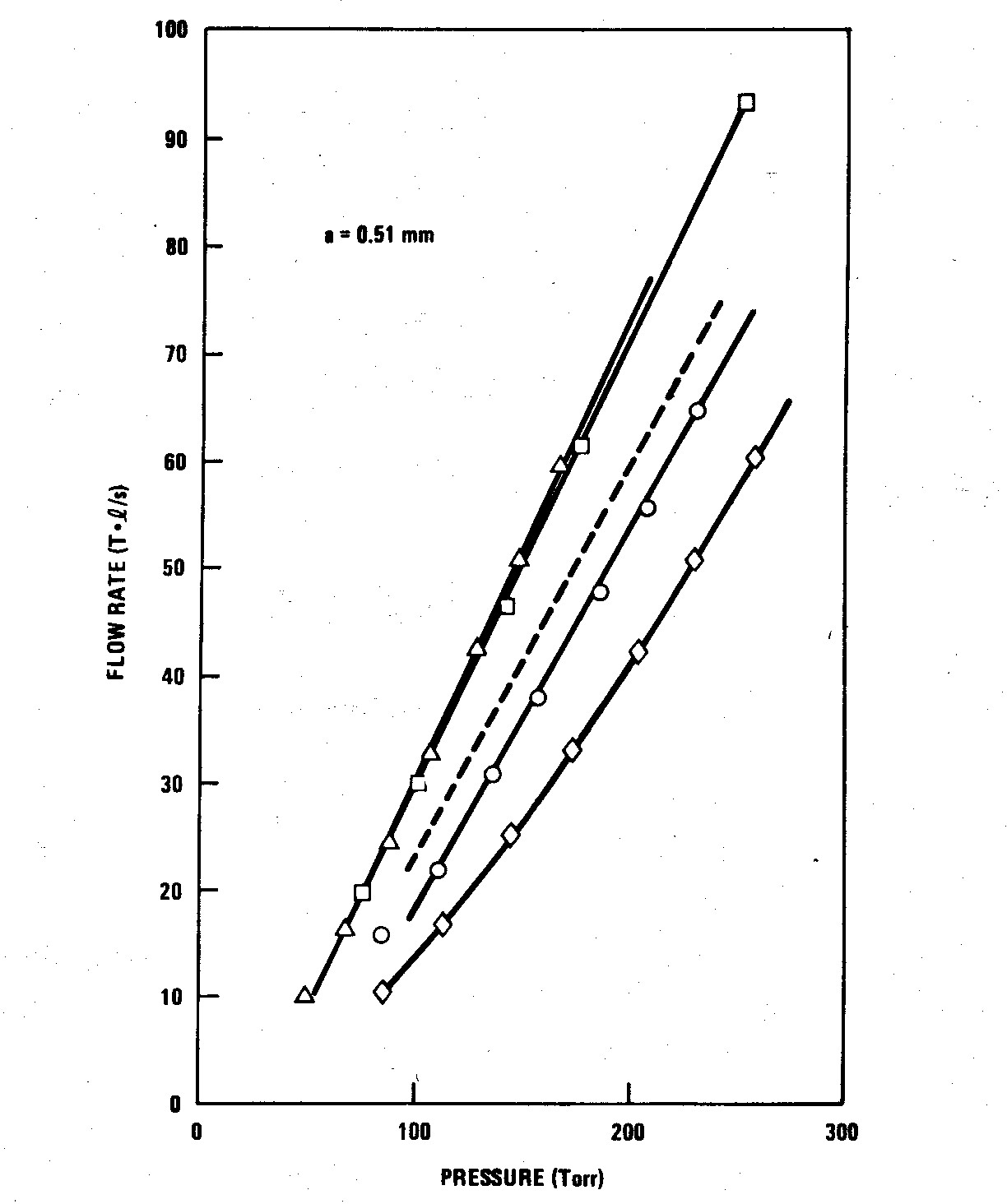
FIG. 6. Flow rate vs pressure for various tube lengths but constant tube radius (a = 0.508 mm). Pressure measured is stagnation pressure except where otherwise indicated. ∆ℓ = 35.5 mm; □ℓ = 70 mm static pressure; --ℓ = 70 mm stagnation; Oℓ = 89 mm; ○ℓ= 151 mm.

For a pressure transducer that measures static pressure the ratio of the slopes of the Q vs p relationship can be derived from Eqs. (11) and (12),

S₁/S_{2 =} [(m₂/m₁)(γ₁/γ₂)(γ₁+ 1)/(γ ₂ + 1)]^1/2 x [A_t1/A_t2] x

[(2/(γ₁+1))(1+ ((γ - 1)/2) M₁²)] ^{γ1/( γ1-1)}/ [(2/(γ₂ + 1))( 1+ ((γ₂ - 1)/2) M₂²)] ^{γ2/( γ2-1)}

In deriving this equation, one must recall that the data in Figs. 3-6 are in terms of particle flow rate, while Eq. (11) is in terms of mass flow rate. This equation can be used to predict the variation of the slopes with m and y.

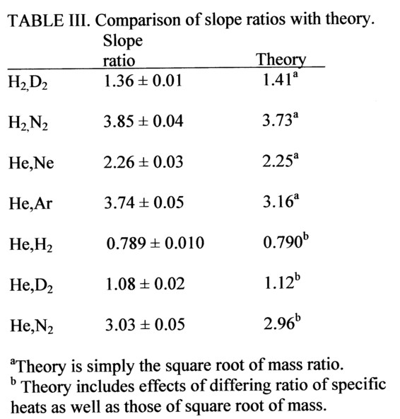
Consider first a group of gases (either monatomic or diatomic) with the same γ. Assuming A, is constant, Eq. (14) predicts that the ratio of the slopes S of the data in Fig. 4 should be given approximately by S₁/S₂ = (m₂/m₁)^1/2 . Table III shows that this expectation matches the data to within about 10%. The remaining discrepancy may be due to small variations in Mach number M and in effective area A, of the sonic orifice as gas type is varied.

In order to compare monatomic with diatomic gases we must have some estimate of the Mach number M. From the hydrogen gas data in Fig. 5, we see that the ratio of p_o/p_s is 1.40. (Compare, for example, the static versus stagnation pressure data for the 12-mm length tubes.) This implies Mach number M ~ 0.71. If we use this value in Eq. (14), we find the values of the helium-to-hydrogen slope ratio given in the lower part of Table III. The agreement with the experimental value is within a few percent.

One final feature of the data that is understandable simply from the sonic orifice condition is the variation in the flow with tube area. The slope of the flow rate versus pressure data should be proportional to tube radius squared. The slopes of the data in Fig. 6 are twice those in Fig. 5;the α² ratio is 2.0. [This conclusion of α² scaling should hold true even when boundary layer thickness is appreciable, since Eqs. (1) and (2) imply that δ * is proportional to α at a fixed flow rate Q_m.]

Although the qualitative features of the flow appear to dominated solely by the physics of the sonic orifice, an attempt to quantitatively predict the flow rate from Eq. (11) reveals that the growth of the boundary layer down the tube also has a significant effect on the flow. Flow rates are a factor of 0.5 to 0.7 below those that would result from a sonic orifice with the full tube radius.

We can check to see whether such a reduction is reasonable by comparing the boundary layer thickness deduced from the throughput reduction to that predicted by Eq. (2). Before this is done, we need to be sure that Eq. (2) applies, i.e, that the flow is in the early stages of the boundary layer development. From Eq. (9), using a hydrogen flow of 100 Torr liter/s in the α= 0.36-mm tube, we find l_t = 20 cm; this corresponds to σ_t = 1. 7 X 10^-2 for the 30-mm length tube. Accordingly, the flow is indeed in the early stages of transition.

From Eqs. (1) and (2), we can estimate δ*. Remembering that the boundary layer grows over the full length of the tube, we find δ * = 0. 13 mm (i.e., δ*/α = 0.37) for a hydrogen flow of 60 Torr liter/s in the 30.4-mm-long, 0.36-mm radius injector. Using the slope of the 1 = 30.4-mm tube data from Fig. 5 plus Eq. (11), we find an effective area that is 63% of the geometrical tube area. This implies δ*/α = 0.2.

Although the boundary layer thickness computed these two different ways are of similar magnitude, it is difficult to make the theory much more quantitative. This is because Eq. (2) is a formula for boundary layer thickness in the case of a flat plate with uniform flow in the free fluid away from the plate. In the tube of the gas injectors, however, the constriction of the flow causes an acceleration. In addition, the sonic jet at the end of the tube means that the flow in the tube is rapid enough that compressibility effects are probably important. (Accordingly, incompressible flow calculations [5],[7] are not adequate.) Both these effects make it difficult to extend the model to make quantitative predictions of flow rate.

A peculiarity of this flow is the lack of dependence on viscosity. The data include gases with viscosities [8] that vary by a factor of 3.5. Consequently, one might expect some effect on the boundary layer growth. However, although the boundary layer may grow at a different rate, it appears that, once it begins to constrict the flow channel, the core acceleration in response to this causes the growth to saturate, thus producing almost equal effective areas for various gases. Indeed, a boundary layer thickness that is independent of flow rate and, at best, weakly dependent on viscosity is what is needed to explain the data.

One final peculiarity of the flow is that, while the linearity of the data in Eqs. (3)-(6) is consistent with the sonic orifice condition Eq. (11), the nonzero intercepts of the various data groups are not. This offset is probably due to the pressure drop in the tube. However, if this is the case, this drop must be essentially independent of flow rate. For most of the tubes studied, the offset does increase with tube length (cf. Figs. 5 and 6) and finally begins to show some flow dependence for the longest tubes. A pressure drop that is flow rate independent is consistent with Eq. (5) and our previous observations that к and δ * are flow rate independent.

In conclusion, our model of sonic orifice flow modified by a wall boundary layer encompasses most of the essential physics. The linearity of the flow rate versus pressure data, the changes in the slopes with working gas mass and specific heat ratio as well as the quadratic scaling of throughput with tube radius all follow quite naturally from Eq. (11). However, owing to the difficulty of describing the boundary layer growth quantitatively in an accelerating, compressible flow, the only way at present to accurately determine the flow rate versus pressure relationship is through actual calibration experiments.

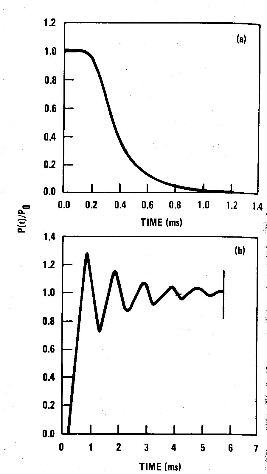
Figure 7. (a) Decay of gas injector pressure sensor signal after voltage shut off (at t = 0);) b) rise of gas injector pressure sensor signal after voltage turn on (at t = 0). Test gas is hydrogen in both cases.

ACKNOWLEDGMENTS

This work was supported by the United States Department of Energy, Contract No. DE-AT'03-76ET5 1011.

a. S.C. Bates and K.H. Burrell, Rev. Sci. Instrum., 55 (6), 938-939, (1984)

1. K. H. Burrell, Rev. Sci. Instrum. 49, 948 (1978).

2. H. F. Dylla, J. Vac. Sci. Technol. 20, 119 (1982).

3. L. D. Landau and E. M. Lifshitz, FluidMechanics (Pergamon, New York, 1959), pp. 148-149.

4. S. Dushman, Scientific Foundations of Vacuum Technique, 2nd ed. (Wiley, New York, 1962), p. 82.

5. H. L. Langhaar, J. Appl. Mech. 9, A-55 (1942).

6. R. H. Sabersky, A. J. Acosta, and E. G. Hauptmann, RuidKow, 2nd ed. (MacMillan, New York, 197 1), Chap. 8.

7. E. M. Sparrow, S. H. Lin, and T. S. Lundgren, Phys. Fluids 7, 338 (1964).

8. Dushman, Scientific Foundations of Vacuum Technique, 2nd ed. (Wiley, New York, 1962), pp. 16, 32.

Home