A displaced line velocity diagnostic and its application in a visualization engine
40 Nutmeg Lane
Glastonbury, CT 06033
ABSTRACT
A technique for measuring three dimensional velocity by imaging the displacement of a marked fluid line is described, together with its use in an automotive visualization engine. In a flow seeded with 2 3 µ phosphorescing particles, a line is excited by a UV laser beam, deformed by the local velocity field, and detected by stereo low light level video cameras. The derivation of velocity from digitized images is discussed and capabilities of the diagnostic are assessed. Some image data taken in the engine are shown and quantitative two component velocity plots along the line are presented.
List of symbols
| C | capacitance |
| dc(s) | displacement of line center |
| e | exponential |
| E | light energy |
| Ef | fractional energy emitted |
| I | light intensity |
| r | position vector |
| s | arc length |
| t | time |
| V | velocity |
| V | voltage |
| x | cartesian position |
| Y | cartesian position |
| Z | cartesian position |
| Δv | change in velocity |
| τ | phosphor lifetime |
Subscripts
| c | line center |
| d | displacement |
| o | original, at time of laser firing |
| r | position |
1 Introduction
The measurement of velocity in a turbulent flow field can be performed in many ways, but the most appropriate diagnostic technique to use depends on both the physical context of the particular flow and the type of velocity information needed. The highly three dimensional and chaotic nature of the flow make it difficult to deduce the whole flow field from measurements taken at a point or even from an entire plane within the flow. Additional complications arise from the need to know the instantaneous flow field, rather than its statistical description.
In this work a diagnostic is described that detects the flow velocity at a line inside the volume, based on a column of optically excited marker particles that have been displaced by the flow. Examining flows by marking a fluid element is a very old technique. Smoke or dye markers were used in some of the first flow visualization work. Most often these markers were used to show streamlines or streaklines in the flow or to illustrate velocity profiles in steady flows. Practical markers included mist, dyes, smoke, or bubbles any tracer that followed the flow (Merzkirch 1974). One recent experiment (Hamamoto et al. 1985) used a smoke wire in the cylinder of an engine to give qualitative information about characteristics of the swirl. Other work has been done with luminescent vapors in gaseous flows (Epstein 1972; Bates 1977), and there has been some use of photochromic chemicals in liquid flow (Falco and Chu 1987).
The problem of interest in this work is to determine the velocity field in an intermittent turbulent internal flow: specifically, the flow inside the cylinder of a spark ignited fourstroke internal combustion engine. Information about this flow is needed because the flow field shapes the combustion, and the combustion determines various important performance parameters of the engine. There are severe constraints for a diagnostic in this case because the total volume is small (<1000 cm3) and the measurement device and the access needed to use it must not disturb the flow. As a result, recent work (Peterson 1979; Lederman and Sacks 1984; Bechtel and Chraplyvy 1982) has emphasized diagnostics that only interact optically with the measurement volume in the engine.
A dedicated visualization engine facility has been built to provide optical access to this internal flow (Bates 1988). It uses a transparent cylinder wall and a piston top window to maximize access for a variety of optical diagnostics that can be used to measure the physical processes that take place inside the cylinder. The diplaced line diagnostic was developed specifically for use in this engine.
2 Displaced-line velocity diagnostic
2.1 Diagnostic concept
A line is optically marked in the flow in a time that is short compared with characteristic flow times. The marking persists, causing the line to remain visible as it is distorted by the local flow field (Fig. 1). The displacement of the line is used to deduce the velocity along the line.
Experimentally, in a flow seeded with phosphorescent particles, a laser is used to excite a line that is later recorded by stereo video cameras to give its three-dimensional change in position. The images are then digitized and analyzed for a continuous record of velocity along the line. The line can be directed through any region of interest in the flow.
Multiple laser pulses and lines can be used to examine in greater detail the full three-dimensional flow field and its time development.
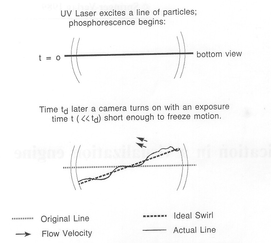
Fig. 1. Displaced-line velocity diagnostic schematic.
2.2 Velocity derivation
The experimental data used to determine velocity are a pair of two-dimensional images of the displaced line together with reference images of the initial line. Two images together form a stereo pair from which the three-dimensional velocity can be derived.
The basic parameter used to calculate velocity is the displacement of the center of the line, dc(s), where s is the arclength along the line. The arclength along the distorted line is longer than the original straight line and the line has a finite width, w(s). The diplacement time, td, is chosen to give an appropriate displacement of the line for the velocity range of the flow; td, is set experimentally and known accurately.
The line displacement is a result of the velocity of the flow in which the line is embedded.
The line-center displacement and displacement time together define a velocity

This velocity is a space and time averaged velocity. It is a meaningful descriptor of the flow in itself, but it is not related exactly to the instantaneous velocity or the mean or turbulent velocities at a point in the flow. The line-center average velocity includes changes that have occurred over the displacement interval:
This is a decomposition of the velocity Vc into the velocity at the original line, Vo, at t = 0, plus the change of the original velocity over space, ΔVr(r, t = 0), plus the change of the velocity field with time ΔVr(r, t). By treating the velocity in this way, the accuracy of the typical case can be assessed when V, closely approximates the initial velocity.
Equation (3) defines the problem as a superposition of steady and unsteady velocity fields rather than mean and turbulent velocity. This approach is one choice for analyzing a flow where unsteady time and length scales overlap turbulence scales. The initial velocity is then
In regions of large spatial gradient of velocity over the distance of line movement, or large temporal variation during the time of the displacement of the line, the velocity at the original line position cannot be deduced accurately. These time and space variations can often be seen by variations in the intensity profile of the displaced line.
Overall, the approximations used to derive velocities from displaced-line images consist of three main types: particle lag approximations, velocity field approximations, and geometric approximations. Particle lag is made negligible by using small enough particles, and velocity approximations are submerged in the use of an encompassing average velocity.
Geometric approximations arise from defining the displacement of a diffused, distorted, thick line. The initial condition of this line is clearly specified and the gross movement of the line is set by the movement of its center, but knowledge of the line center position is only approximate due to a lack of knowledge about the internal motion of the line. Since particles can be rearranged within the two-dimensional image of the line, incorrect velocities can be derived by assuming proportional mapping of points along the line.
Information relevant to the refinement of all these approximations is contained in the detailed distortion of the displaced line. The change in thickness and intensity of the line is a measure of the velocity gradients on that scale. A varying velocity component parallel to the line causes changes in intensity along the line. These effects are complex and can be ambiguous due to the multiplicity of ways that the final line distortion can be achieved. Experience with the technique will clarify what details can be learned about the velocity from experimental line images.
2.3 Technique optimization
In order to diagnose the full, instantaneous, three-dimensional velocity field more than just a single line is required. A fine, three-dimensional, orthogonal grid would be best conceptually, but such a grid is impractical for a variety of reasons. The major fundamental limit to using a set of lines in the flow is that they must be separable in both camera views after they have been displaced. This is a severe limitation because of other experimental constraints: the lines have finite width, the images have limited resolution given that the whole flow field must be included (especially video), and the best depth perception occurs for orthogonal camera viewing directions. The combination of these conditions results in a requirement that there be a limited number of lines, forming a relatively coarse network. The lines may even have to be non-orthogonal. To explore these various effects in an uncomplicated manner the technique is being developed using a single line.
Optimizing the experimental line thickness is also not simple. The best line thickness is determined from the consequences of the turbulence length scales and image resolution. The line should be 10 or more pixels wide for the most accurate determination of the line center. The line thickness sets the degree of averaging over the smallest turbulence length scales, thus for average flow measurements a thicker line is easier to analyze and will not decrease in intensity due to dispersion of the particles by turbulence. However, for small scale turbulence measurements, the line width should be at most the Kolmogorov length scale of the flow. Such turbulence measurements are Eulerian, embedded in the flow as the line is, and thus different than most data taken in turbulent flows.
2.4 Application assessment
The displaced-line technique is designed to give first order velocity information from complex three-dimensional flows. It represents a compromise between the need for massive amounts of data to understand a highly three-dimensional flow and the requirement that there be a manageable amount of information derived from experimental techniques that are not extremely difficult.
The primary advantage of the displaced-line technique is that it gives a spatially continuous record of the velocity along an arbitrary line (or lines) in the flow. These lines can also be re-marked at a later time without interference from previous measurements. The main disadvantage of the technique is that the derived velocity is in most cases an average that submerges some of the details of the turbulent flow.
The requirements for this displaced-line technique are optical access for both excitation and imaging, a suitable marker, plus image recording and digitizing equipment. The low light output from the phosphor will limit its application primarily to laboratory work, but within that context the technique can be used for most flows.
3 Experimental technique
3.1 Diagnostic process overview
The diagnostic process uses optical energy to measure a very specific property of a flow. The components of the technique, as well as their feasibility and efficiency, can be examined by detailing the process as it progresses from the laser to the video output. Many parts of the process are independent and can be measured and optimized separately.
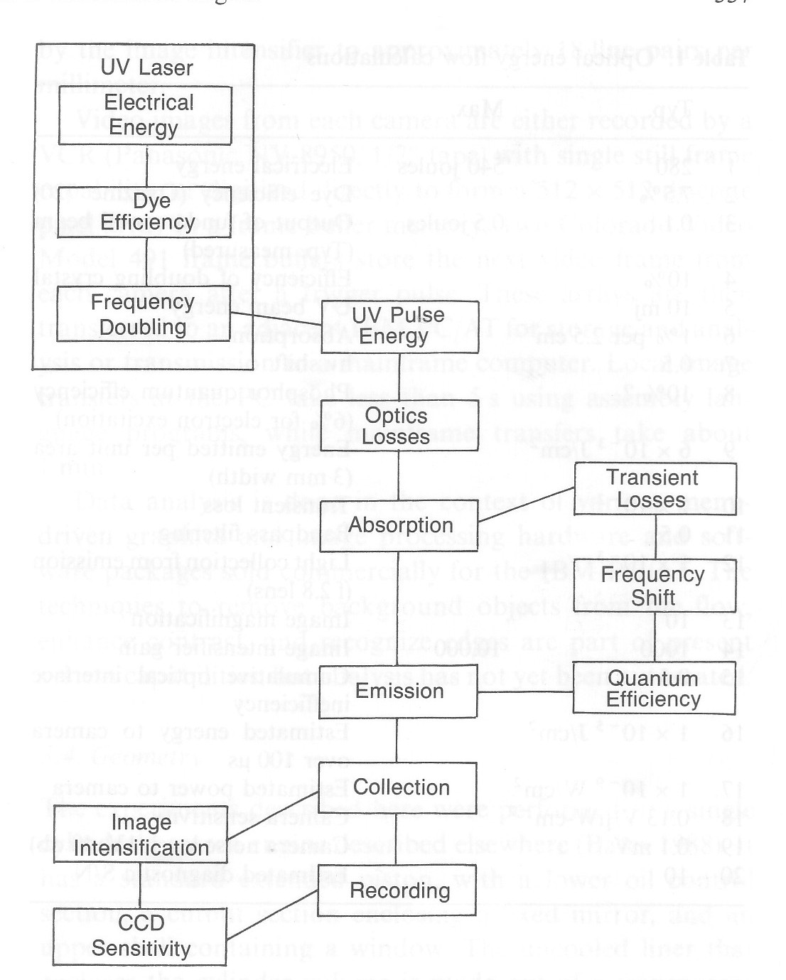
Fig. 2. Light energy flow chart.
An energy flow block diagram of the entire photo-optical exciting and recording system is shown schematically in Fig. 2. The process is conveniently separated into laser pulse production, phosphor absorption and emission, and image light collection and recording. The numbers appropriate to the various processes indicated are given in Table 1.
The line marked in the flow is excited by a Candela flashlamp-pumped dye laser that is frequency doubled into the near UV. There are two lasers, and while both have a low repetition rate (2 pps) they can be triggered to operate nearly simultaneously with a variable delay to examine events that develop rapidly. Using oxazine 720 dye in a pure methanol solution, the laser output is in the form of 1/2 microsecond pulses centered at 350 run. Oxazine 720 was chosen because it had the highest efficiency (7.5%) of the dyes that have a frequency doubled output in the near UV. The multimode laser beam is 1 cm diameter at the laser, and is transferred to the engine by UV mirrors, where it is focussed down to a few millimeters.
To calculate the total energy per unit area absorbed, it is assumed that the particle density is adjusted to give 1 % per 25 min absorption of the laser beam so that the absorption is a maximum, while remaining linear as a function of path length. This represents a 4% decrease in beam intensity per pass through the cylinder.
The efficiency of the absorption and emission of light from the phosphor is given by a phosphorescence quantum efficiency, which represents the fraction of photons out per photons in. For phosphor particles this has only been measured using electron excitation, but it can be estimated as being between electron excitation of particles and UV excitation of gases: 10 %. A further factor is the decreased energy of the green output photon as compared to the input UV photon (line 7).
The phosphorescence decays with time at an exponential rate characterized by the lifetime as shown in Table 1. Transient losses result from the fractional energy Ef collected for a previously defined line displacement interval as discussed below. These are estimated by an Ef of 1 % (line 10).
Collection of the phosphorescence is done by a commercial 35 mm camera lens with f2.8 optics. Some of the light losses per unit area of collection are regained due to the image reduction of the 100 turn square object onto the 10 min square area of the image intensifier face. The image intensifier itself provides a maximum photon gain of 104 and a typical operating gain of 103.
The overall energy transmitted to the camera in 100 µs is the combination of estimates in lines 9-15: 10-5 J/cm2. This represents an average power of 10 - 9 W. The nominal sensitivity of the camera is 0.1 V/µW-cm-2 with a typical noise level of 0.1 mV (I V, 40 db signal to noise). This implies an image signal to noise ratio of 10.
| Typ. | Max. | ||
|---|---|---|---|
| 1 | 280 | 540 joules | Electrical energy |
| 2 | 7.5% | Dye efficiency (Oxazine 720) | |
| 3 | 0.1 | 0.5 joules | Output of fundamental beam (Typ. measured) |
| 4 | 10% | Efficiency of doubling crystal | |
| 5 | 10 mj | UV beam energy | |
| 6 | 1% per 2.5 cm | Absorption | |
| 7 | 0.5 | hv shift | |
| 8 | 10% ? | Phosphor quantum efficiency (6% for electron excitation) | |
| 9 | 6 x 10⁻³ J/cm2 | Energy emitted per unit area (3 min width) | |
| 10 | 1 x 10⁻² | Transient loss | |
| 11 | 0.5 | Bandpass filtering | |
| 12 | 1 x 10⁻³ | Light collection from emission (f 2.8 lens) | |
| 13 | 10 | Image magnification | |
| 14 | 1000 | 10,000 | Image intensifier gain |
| 15 | 0.5 | Cumulative optical interface inefficiency | |
| 16 | 1 x 10⁻⁵ J/cm2 | Estimated energy to camera over 100 µs | |
| 17 | 1 x 10⁻⁹ W/cm2 | Estimated power to camera | |
| 18 | 0.13 V/µW-cm-2 | Camera sensitivity | |
| 19 | 0.1 mV | Camera noise level (1V: 40 db) | |
| 20 | 10 | Estimated diagnostic S/N |
3.2 Phosphor tracer and seeding
The use of phosphorescent particles as a fluid marker is a recent innovation. While the phosphorescence of solids has a long scientific history (Goldberg 1966), almost all of the studies of these materials have used electron excitation rather than excitation by UV radiation (Anderson and Ricchio 1973). This paper describes work with phosphor powders in progress since 1984. Totally independent work in Japan involving a simpler 2-d version of a displaced-line technique has recently been reported (Nakatani and Yamada 1986).
The most significant characteristics of a phosphor as a tracer are the wavelength of its emission peak, its emission lifetime, and its mean diameter. Available lifetimes vary by a factor of 107, so the emission can be tailored to the application in both wavelength and output energy. Another important parameter is energy transfer efficiency, which indicates how much of the incoming optical energy is lost before the particle emits it as phosphorescence. There are many quantum losses in the decay of the excited state to the emitting singlet or triplet state, and while the energy reemitted can be as large as 20%, for practical phosphors it typically varies between 1%-15% depending on the compound involved.
Although a gas would be a superior phosphorescing tracer for flow tracking, the phosphorescent emission from the excited triplet state of the gas molecule is quenched by oxygen, thus such a gas is not compatible with air-breathing engine studies. Solid phosphorescence is an internal lattice phenomenon not subject to collisional quenching.
The commercially available phosphor particles were seeded into the flow by a fluidized bed aerosol generator, TS1 Model 9310. This aerosol generator nominally produces 5-15 l/min of seeded flow, with a particle concentration of 105-106 per cm3. The seed concentration used experimentally was near the lower limit. A particle size of 2-3 µ was chosen to be sure that the particles follow the flow in an internal combustion engine. The seed flow was continuous past the intake port, drawn into the engine during the intake process.
Subsidiary properties of the phosphor particles are that they do not scratch glass and are chemically inert. However, some of the compounds are toxic. It is not known if they will survive combustion in the engine.
3.3 Image equipment and image handling
The phosphorescence from the seeded flow is recorded with low-light-level video cameras. The cameras are image intensified Fairchild CCD video cameras made by ITT, with a microchannel plate image intensifier directly attached to the CCD array by a fiber optic plate. The camera output is linear, with a dynamic range of approximately 1000. The image intensifier is an 18 min diameter single stage device that provides a non-linear luminous gain adjustable to a maximum of 10,000. The image intensifier can also be gated by a 5 V pulse as short as 1 µs at a repetition rate of up to 3000 Hz. This allows fast shuttering of the camera for instantaneous images during engine operation. Camera output is fixed at 30 frames per second (NTSC video) by the high data rates needed to scan the 380 x 480 element CCD array. The image resolution of the camera system is limited by the image intensifier to approximately 18 line pairs per millimeter.
Video images from each camera are either recorded by a VCR (Panasonic NV-8950, 1/2" tape) with single still frame capability, or digitized directly to form a 512 x 512 discrete pixel array in a frame buffer memory. Two Colorado Video Model 491 frame buffers store the next video frame from each camera after a trigger pulse. These arrays are then transferred to an adjacent IBM PC/AT for storage and analysis or transmission to a mainframe computer. Local image transfers at the PC take less than 5 s using assembly language programs, while mainframe transfers take about I min.
Data analysis is done in the context of various menu driven graphics and image processing hardware and software packages sold commercially for the IBM PC/AT. The techniques to remove background objects from the flow, enhance contrast, and recognize edges are part of present system capabilities, but analysis has not yet been automated.
3.4 Geometry
The experiments described here were performed in a single cylinder research engine described elsewhere (Bates 1988). It has a standard extended piston, with a lower oil control section, a cutout section enclosing a fixed mirror, and an upper shell containing a window. The uncooled liner that encloses the cylinder volume is made out of a transparent material such as glass, plastic, or sapphire, and extends up to the bottom of the head so that there is 360o optical access to the entire engine chamber. The head includes overhead cams, two intake valves, one exhaust valve, and two spark plugs in a shallow cavity typical of current automobile technology. The head is attached to the engine body with thin high-strength posts set away from the liner. This geometry is shown in Fig. 3 a and b, with a schematic diagnostic line superimposed.
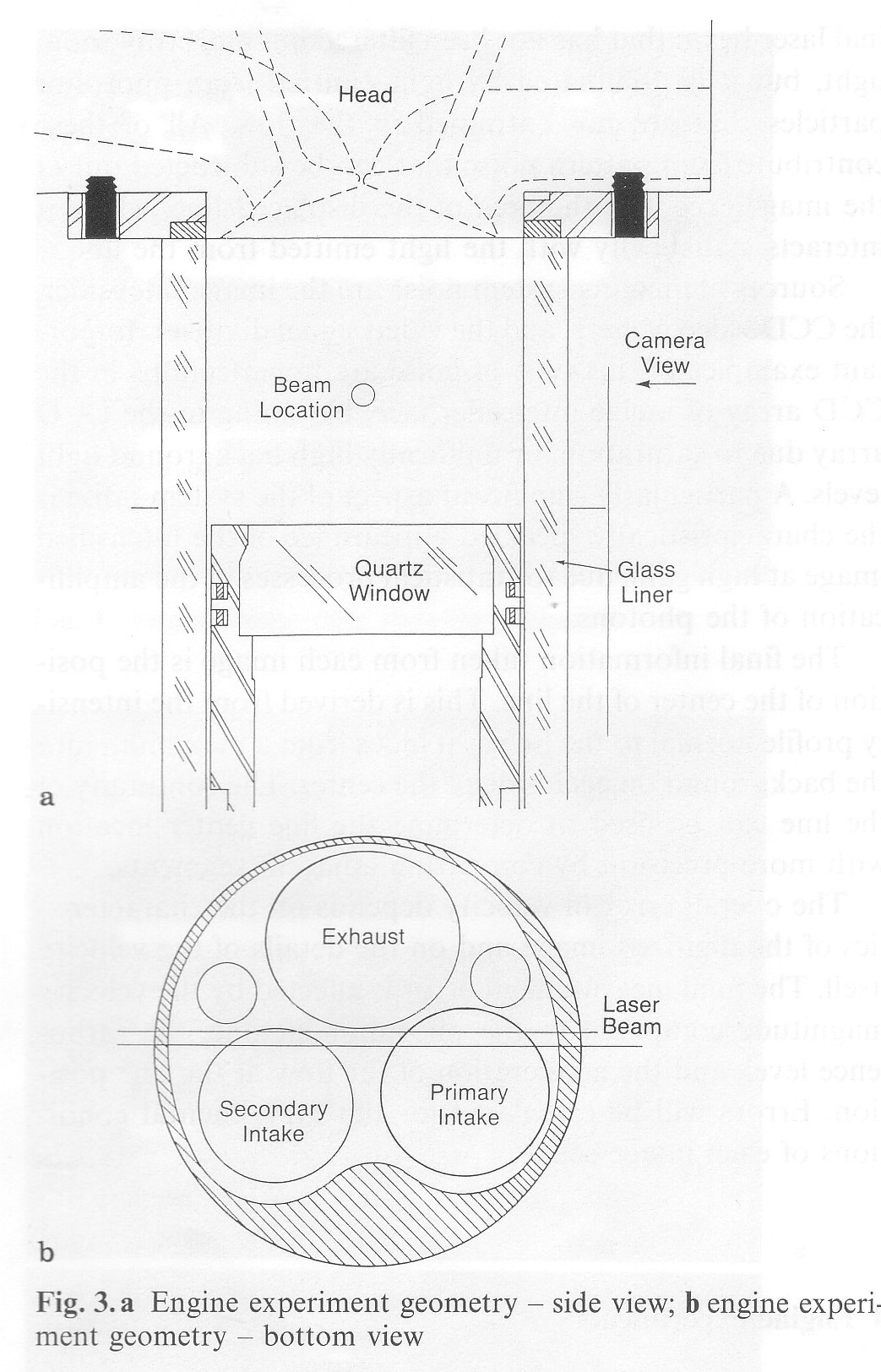
For the data described here, the stereo cameras both look through the cylinder wall from different angles. The view of one is indicated in Fig. 3 a, while the view from the other is similar to that shown in Fig. 3 a, except that this camera is slanted to look up from below the level of the piston-top into the head cavity. For events very near top-dead-center of the cycle both views must be taken up through the piston-top window.
3.5 Experiment timing
Flow visualization experiments are timed with respect to engine operation such that laser firing and camera gating are done at a fixed crank angle. The engine cycle timing is based on a shaft angle encoder (0.1° accuracy) attached to the crankshaft. Within the CCD camera, photons from a gated image are summed in each cell until the change is rapidly stored in transfer registers, from which that video frame is scanned and transmitted. The frame buffers have been triggered to capture this image. Due to this internal sequencing it is not necessary to synchronize the camera and the exposure.
The timing of the camera gating relative to the laser pulse is an important parameter. The decay of the phosphorescence is exponential
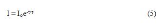
where I is the radiated intensity, I, is the intensity at t = 0, and r is the phosphor lifetime. The total energy, E, emitted in an interval that begins at t, and ends at t, is
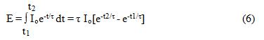
Since the total energy emitted depends on the absorbed energy and not the phosphor lifetime, a more appropriate quantity to optimize for captured energy is the fraction of energy, Ef, emitted in the interval. The phosphor lifetime is chosen to extend over a period that allows the emitting line to move, but the exposure interval must be much shorter to make an instantaneous image of the line. Thus, (t2 - t1) << T and
The energy captured is not only linearly dependent on the length of the interval, as expected, but also depends on how close to the laser pulse the interval is set, as measured relative to the phosphor lifetime. For typical parameters τ = 2 ms, t1 = 1.32 ms, and t2 = 1.58 ms, Ef ≈ 7%. Care must be taken to maximize this fractional energy within the constraints of the experiment.
3.6 Diagnostic reference image
The reference data of the displaced-line diagnostic is an image of the seeded flow that is taken during a very short interval that includes the laser pulse itself. This image will include the undisturbed beam geometry and the background noise that can be subtracted from the data images with image processing. The information contained in this image, together with the parameters that are used to set up the engine, provide the data needed to reproduce any experiment.
3.7 Velocity error and system noise
The total error in flow velocity derived from images of displaced lines has its source in image noise, geometric inexactness, and the velocity approximations described above.
Noise in the image becomes velocity error when the image is processed to find the line displacement. This noise combines inaccuracies in the digitization of the analog video signal, noise in the imaging system itself, and noise that is part of the image light entering the lens of the camera. Image light noise arises partially from scattered light from the original laser beam that has not been filtered out and stray room light, but it is dominated by light emitted from phosphor particles that are not entrained in the flow. All of these contribute fixed pattern noise that can be subtracted out of the image except in the area of the displaced line, where it interacts statistically with the light emitted from the line.
Sources of imaging system noise are the image intensifier, the CCD video camera, and the video signal digitizer. Important examples of this type of noise are imperfections in the CCD array of image intensifier face, blooming in the CCD array due to saturation, or uniformly high background light levels. A particularly significant aspect of the system noise is the characteristically speckled appearance of the intensified image at high gain, due to statistical processes in the amplification of the photons.
The final information taken from each image is the position of the center of the line. This is derived from the intensity profile normal to the line as it fades from a maximum into the background on each side of the center. The continuity of the line can be used to determine the line center location with more precision by comparing adjacent segments.
The overall error in velocity depends on the characteristics of the digitized image and on the details of the velocity itself. The final measurement error is affected by the velocity magnitude compared to the phosphor lifetime, the turbulence level, and the acceleration of the flow at the line position. Errors will be calculated for the experimental conditions of each image set.
4 Engine experiments
The data described here were taken in the visualization engine set up with a 1/2" thick glass liner. The engine bore and stroke are 92 mm. All of the data shown here were from experiments conducted at 500 r/min and open throttle, with no flow through the secondary intake port.
There is only one pass of the beam through the cylinder (Fig. 3 a and b) to minimize internal reflections of the UV laser beam from the inner wall. The beam intersects the cylinder axis so that the reflected beam is superimposed on the incident beam, except for the focussing due to the convex wall.
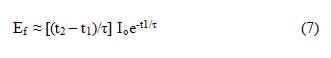
For the camera view noted in Fig. 3 a, Fig. 4 shows a reference image of the engine geometry. The brightest part of the image comes from the phosphor particles excited directly by the laser beam. Background noise has been enhanced to show the laser line relative to the engine components. The piston is clearly visible at the bottom, as is the joint between the head and liner at the top and the upper limit of the ring travel below it. This background noise results from particles attached to all of the interior walls, illuminated by stray UV light. It should be noted that the reproductions of the data shown here do not adequately represent the true image quality, due to the non-linear response of photographic film.
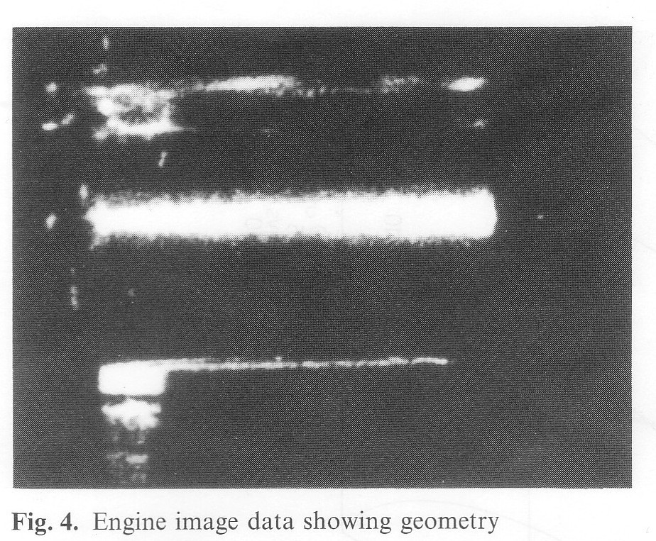
Figure 5 a and b shows reference images of the laser beam geometry and the displaced line at t = 0 for the two cameras from the viewpoints described above. The entrance of the beam on the left and its exit on the right are the brightest spots. The most intense part of the emission from the flow is at the line center, due to line-of-sight integration through the circular beam. The reference images were taken 0. 1° after the laser pulse at 105° crank angle after top-dead-center (ATDC) for an exposure time of 0.1°. For this delay and exposure the flow has not moved since the 1/2 µs laser pulse.
Figure 3 a shows the view seen in Fig. 5 a. The view of the second camera (Fig. 5b) can be more easily visualized by recognizing the two arcs at the top of the image as the joint between the cylinder and the head, and the highest point of the ring travel. The beam enters at the top dot, and its exit lower down in the image is blocked from view by the piston. For these tests, the view through the piston top was not used because phosphor particles accumulated on the window during operation of the engine.
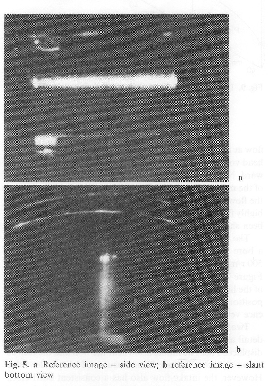
Figure 6 a and b shows the line displaced by the flow during the intake stroke. The imagines were taken at 160° after top dead center (ATDC), 2.0° after the laser pulse, with an exposure time of 0.2°. Figure 7b shows a greater magnification than that of the reference view, but has been calibrated consistently. The original beam entrance and exit are still visible. The beam position is not changed for all of the images data presented, thus they all have the same position relative to the engine as illustrated in the reference images.
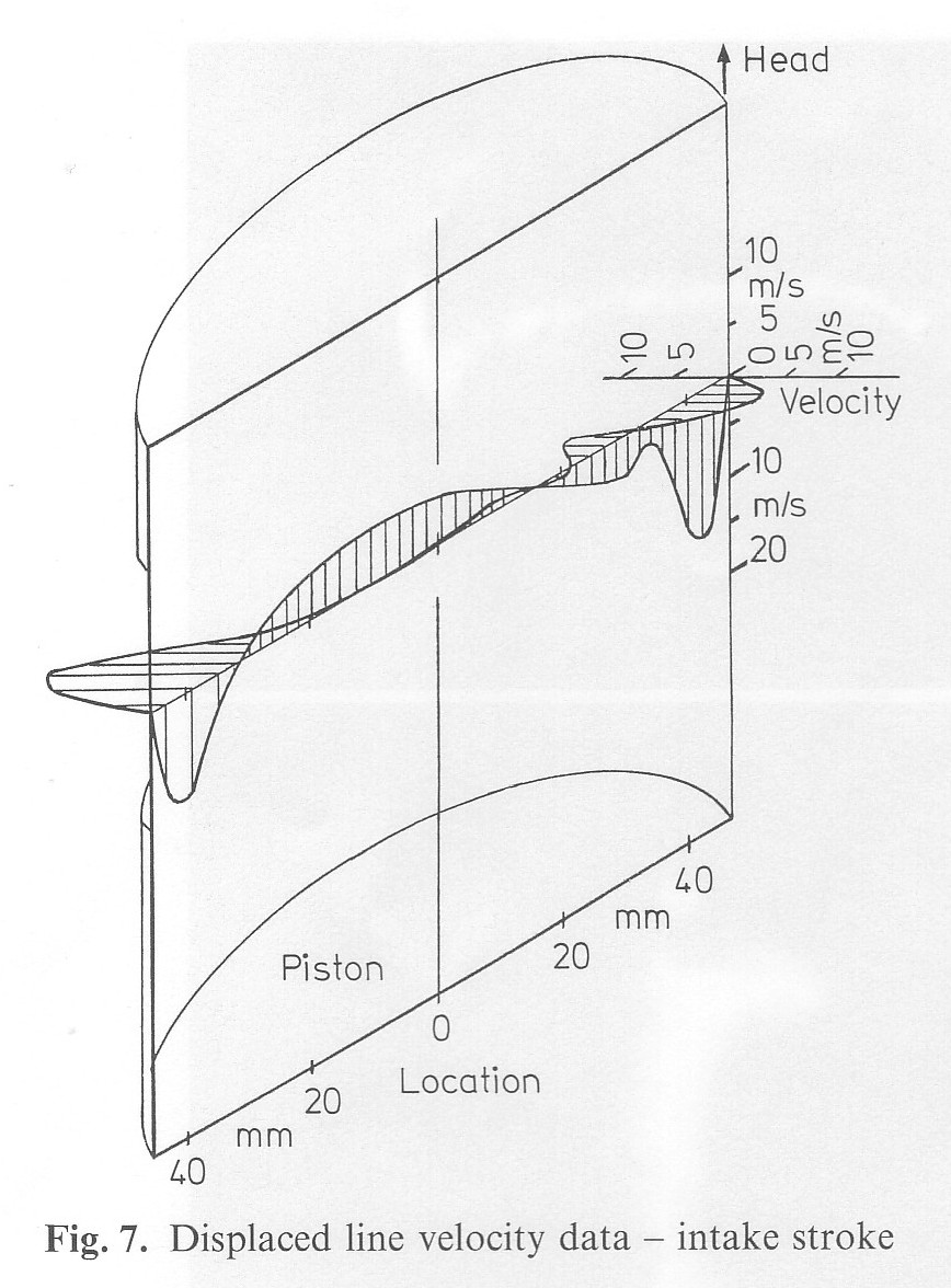
The gross form of the flow is easily seen in Fig. 6a. The large displacements at either side represent slices through the annular jet from the intake valve. The high velocity flow at the right has passed directly down the adjacent wall and thus has higher velocity and is more well defined than thelow at the left, which has had to pass across and through the head volume before hitting the far wall and deflecting downward. Note that the intake valve center is behind the plane of the measurement and slanted. The difficulty of presenting the flow and its geometry in a fixed, flat plot is extreme; the highly three-dimensional geometry of the head itself has only been shown in two planviews.
The velocity is calculated by scaling the image based on a bore of 92 mm and the delay time of 2.1°, or 0.7 ms at 500 r/min. Velocity data from both of the images of Figure 7 a and b are shown in perspective in Fig. 7. The top of the liner and piston are shown for reference relative to the position of the original line. The mean piston speed, a reference velocity for engine work, is 0.8 m/s.
Two orthogonal velocity components that are accurate in detail are shown in Fig. 7, calculated from each view of the displaced line. The intake flows near the wall and the recirculation at the center are basic features of in-cylinder flows. However, the intake flow also has a consistent swirl clockwise from the top of cylinder. This swirl is expected, since the intake port comes straight into the cylinder from behind the side view of Fig. 6 a. A set of data taken at these conditions shows some variation in both the swirl component and the diffusion of the line due to turbulence. The case of Fig. 6 and 7 is one that has more swirl than the average. These changes in flow parameters for identical experimental settings are identified as cycle-by-cycle variation in the engine. The flow is not well enough understood to comment on the other details of the velocity profile that are shown. The magnitude of the velocity, with a maximum of 17 m/s is much reduced from peak intake velocities, since the piston motion has slowed at 20' from BDC and the intake valve is closing.
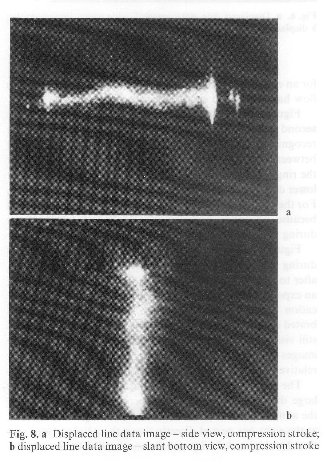
Figure 8 a and b shows the line displaced by the flow in the compression stroke. The images were taken at 20° after bottom-dead-center, again 2.0° after the laser pulse, with an exposure time of 0.2°.
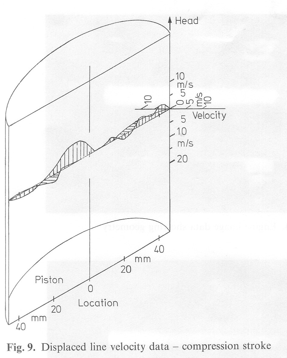
Figure 9 shows the velocities derived from these images. As would be expected, the velocity in the cylinder has decayed from that during the intake flow. The velocity is still usually higher than the mean piston speed, reaching a maximum of 6.9 m/s or almost 9 times mean piston speed. The velocity distribution is indicative of no repeatable flow, and this is confirmed by other image sets. It should be noted that this is a cycle where there is very low swirl; in fact there is a small counterclockwise swirl at this time and cylinder location.
In conclusion, engine cold flow experiments indicate that the displaced-line technique does work adequately for diagnosing in-cylinder velocity. It will be used to examine the development of flow structures and to connect the flow velocity to the development of the flame in each cycle. Improvements in data analysis and presentation will be made as the project proceeds.
5 Discussion
The displaced-line velocity diagnostic has been described both conceptually and experimentally. The diagnostic is a conceptually simple technique using a three-dimensional flow visualization technique made quantitative by the ability to digitize and process the data images. It supplies instantaneous, connected velocity data that seems required to adequately explore turbulent flows, and gives such information in a manageable amount.
The essence of the displaced-line technique is to optically mark a part of the fluid and record images of the marker behavior as a result of motions in the flow. In practice the technique is difficult because sophisticated and expensive equipment is needed when phosphor particles are used as a marker. In order to optimize detector efficiency, excitation must be done with ultraviolet lasers, and even with high energy illumination the emitted light is so dim that special low-light-level cameras must be used.
Important points should be made about the video based imaging system used in this work. The most valuable characteristic of video is immediate output. This allows rapid optimization of equipment parameters and makes the development of techniques like the one discussed here feasible on a short time scale. Furthermore, there are many commercial products available with a wide range of capabilities, including compatible, extensive, and inexpensive image processing systems. One ongoing problem is the lack of an adequate quality (grey scale), inexpensive video hard copy unit, a deficiency from which this work suffers.
The final issue to be discussed is how well the displacedline diagnostic measures the full-field velocity. Certainly the technique is limited in its volume of coverage to the vicinity of the line or lines through the flow field. This is partially compensated for the ability to examine any specific portion of the flow as desired. The ultimate spatial resolution is also limited in some complicated way, however displacements much smaller than practical line widths can be measured easily. The technique should be adequate for generating firstorder information about such complex turbulent flow fields as those in the cylinder of an automotive engine. Fixed secondary flows can be studied at different times with separate lines, while statistical fluctuations of the flow can be assessed in a similar manner over sets of cycles.
A true feeling for the overall value of the technique will only emerge from its further use. At present, the numerical accuracy of the measurement is estimated to be 10%-20% of the mean flow velocity, depending on local conditions. The error is independent of the velocity magnitude, since the experiment is configured to be appropriate to the mean velocity under study. It is increased by velocity parallel to the line and increased turbulent diffusion of the line itself. A more sophisticated analysis of the data will improve this accuracy.
References
Anderson, R. F.; Ricchio, S. G. 1973: Luminescent rise times of inorganic phosphors excited by high intensity ultraviolet light. Appl. Opt. 12, 2751
Bates, S. C. 1977: Luminescent visualization of molecular and turbuleDt transport in a plane shear layer. Gas Turbine Lab Report * 134, MIT, Cambridge/MA
Bates, S. C. 1988: A transparent engine for flow and combustion visualization studies. SAE pap. 880520
Bechtel, J. H.; Chraplyvy, A. R. 1982: Laser diagnostics of flames. combustion products and sprays. Proc. IEEE 70. 658-677
Epstein, A. H. 1972: Fluorescent gaseous tracers for three-dimensional flow visualization. S. M. Thesis, Dept. of Aeronautics and Astronautics, MIT, Cambridge/MA
Falco, R. E.; Chu, C. C. 1987: Measurement of two-dimensional fluid dynamic quantities using a photochromic grid tracing technique. Present at SPIE 31st Annu Symp. Optical and Optoelectronic Applied Science and Engineering, August 16-20, San Diego/CA Goldberg P. (ed.) 1966: Luminescence of organic solids. New York: Academic Press
Hamamoto, Y.; Tomita, E.; Tamura, Y. 1985: The effect of swirl on spark-ignition combustion. Proc. Int. Symp. Diagnostics and Modelling of Combustion in Reciprocating Engines, September 4-6, Tokyo, Japan, 413-422
Lederman, S.; Sacks, S. 1984: Laser diagnostics for flowfields, combustion and MHD applications. AIAA J. 22,161-173
Merzkirch, W. 1974: Flow visualization. New York: Academic Press Nakatani, N.; Yamada, T. 1986: Measurement of velocity and temperature distributions in gas flow by the laser induced luminescence methods. Proc. 4th Int. Symp. Flow Visualization, August 26-29, Paris, France, 179-184
Peterson, C. W. 1979: A survey of the utilitarian aspects of advanced flowfield diagnostic techniques. AIAA J. 17, 1352-1360